Plot graph of direct species associations.
plot.cgr.RdPlot graph of direct species associations.
Arguments
- x
is a cgr object, e.g. from output of
cgr.- P
locations of graph nodes, if NULL (default) these are generated with a Fruchterman Reingold algorithm.
- vary.edge.lwd
is logical, TRUE will vary line width according to the strength of partial correlation, default (FALSE) uses fixed line width.
- edge.col
takes two colours as arguments - the first is the colour used for positive partial correlations, the second is the colour of negative partial correlations.
- label
is a vector of labels to apply to each variable, defaulting to the column names supplied in the data.
- vertex.col
the colour of graph nodes.
- label.cex
is the size of labels.
- edge.lwd
is line width, defaulting to 10*partial correlation when varying edge width, and 4 otherwise.
- edge.lty
is a vector of two integers specifying the line types for positive and negative partial correlations, respectively. Both default to solid lines.
- ...
other parameters to be passed through to plotting gplot, in particular
pad, the amount to pad the plotting range is useful if labels are being clipped. For details see thegplothelp file.
Value
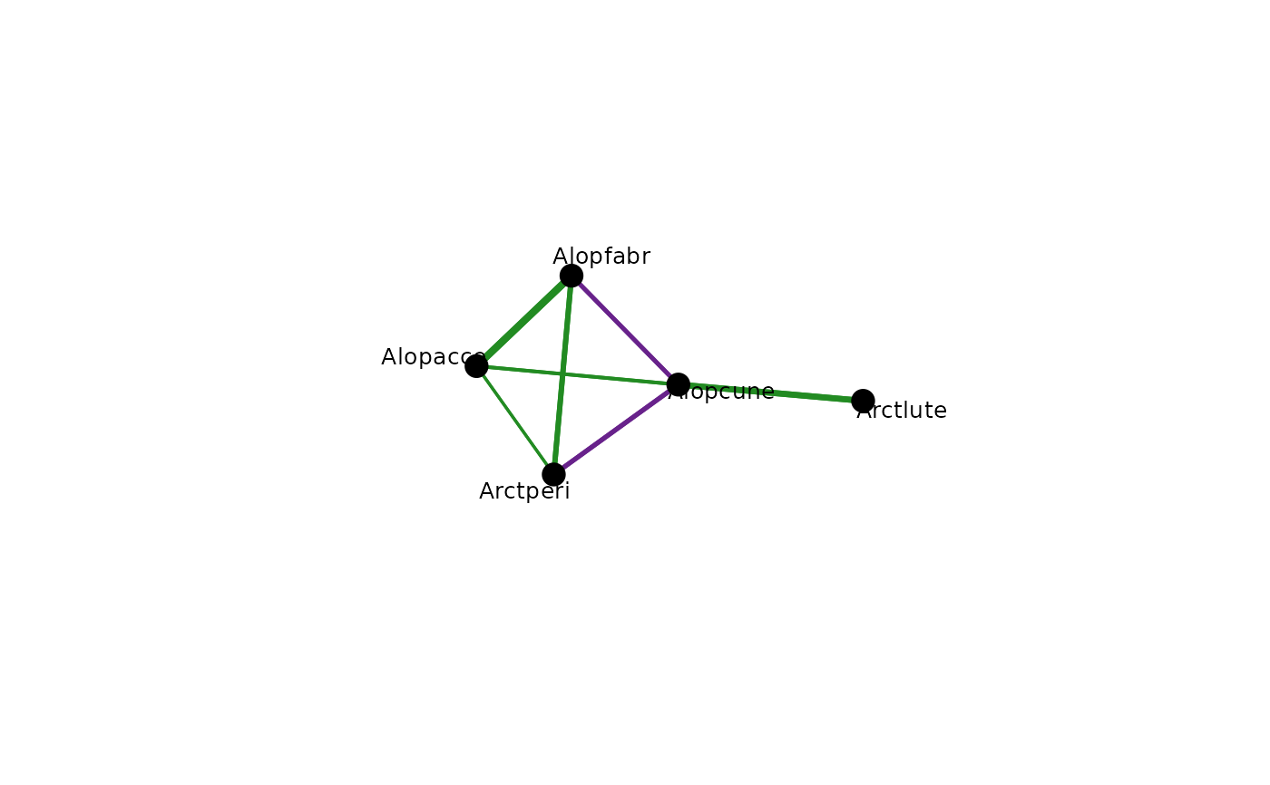
a plot of species associations after accounting for the effect of all other species, positive/negative are blue/pink.
The matrix of node positions (P) is returned silently.
See also
gplot, cgr
Examples
abund <- spider$abund[,1:5]
spider_mod <- stackedsdm(abund,~1, data = spider$x, ncores=2)
spid_graph=cgr(spider_mod)
plot(spid_graph, edge.col=c("forestgreen","darkorchid4"),
vertex.col = "black",vary.edge.lwd=TRUE)
 # \donttest{
library(tidyr)
library(tidygraph)
#>
#> Attaching package: ‘tidygraph’
#> The following object is masked from ‘package:stats’:
#>
#> filter
library(ggraph)
#> Loading required package: ggplot2
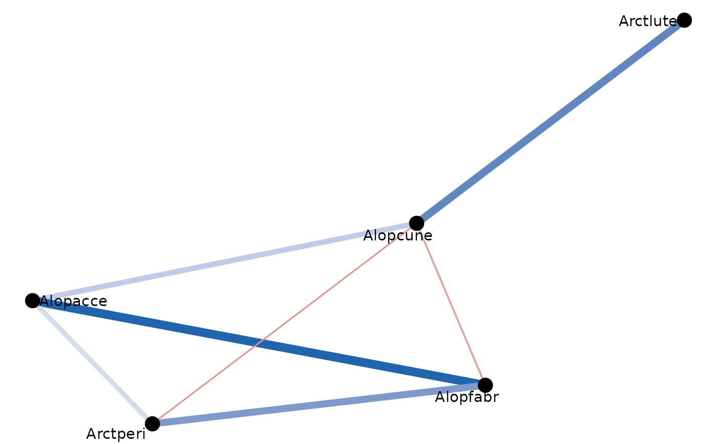
igraph_out<-spid_graph$best_graph$igraph_out
igraph_out %>% ggraph('fr') + # see ?layout_tbl_graph_igraph
geom_edge_fan0(aes( colour = partcor, width=partcor)) +
scale_edge_width(range = c(0.5, 3))+
scale_edge_color_gradient2(low="#b2182b",mid="white",high="#2166ac")+
geom_node_text(aes(label=name), repel = TRUE)+
geom_node_point(aes(size=1.3))+
theme_void() +
theme(legend.position = 'none')
# \donttest{
library(tidyr)
library(tidygraph)
#>
#> Attaching package: ‘tidygraph’
#> The following object is masked from ‘package:stats’:
#>
#> filter
library(ggraph)
#> Loading required package: ggplot2
igraph_out<-spid_graph$best_graph$igraph_out
igraph_out %>% ggraph('fr') + # see ?layout_tbl_graph_igraph
geom_edge_fan0(aes( colour = partcor, width=partcor)) +
scale_edge_width(range = c(0.5, 3))+
scale_edge_color_gradient2(low="#b2182b",mid="white",high="#2166ac")+
geom_node_text(aes(label=name), repel = TRUE)+
geom_node_point(aes(size=1.3))+
theme_void() +
theme(legend.position = 'none')
 # }
# }