Fitting Gaussian copula graphical lasso to co-occurrence data

cgr is used to fit a Gaussian copula graphical model to multivariate discrete data, like species co-occurrence data in ecology. This function fits the model and estimates the shrinkage parameter using BIC. Use plot.cgr to plot the resulting graph.

Usage

cgr(
  obj,
  lambda = NULL,
  n.lambda = 100,
  n.samp = 500,
  method = "BIC",
  seed = NULL
)

Arguments

obj: object of either class manyglm, or manyany with ordinal models clm
lambda: vector, values of shrinkage parameter lambda for model selection (optional, see detail)
n.lambda: integer, number of lambda values for model selection (default = 100), ignored if lambda supplied
n.samp: integer (default = 500), number of sets residuals used for importance sampling (optional, see detail)
method: method for selecting shrinkage parameter lambda, either "BIC" (default) or "AIC"
seed: integer (default = 1), seed for random number generation (optional, see detail)

Value

Three objects are returned; best_graph is a list with parameters for the 'best' graphical model, chosen by the chosen method; all_graphs is a list with likelihood, BIC and AIC for all models along lambda path; obj is the input object.

Details

cgr is used to fit a Gaussian copula graphical model to multivariate discrete data, such as co-occurrence (multi species) data in ecology. The model is estimated using importance sampling with n.samp sets of randomised quantile or "Dunn-Smyth" residuals (Dunn & Smyth 1996), and the glasso package for fitting Gaussian graphical models. Models are fit for a path of values of the shrinkage parameter lambda chosen so that both completely dense and sparse models are fit. The lambda value for the best_graph is chosen by BIC (default) or AIC. The seed is controlled so that models with the same data and different predictors can be compared.

Author(s)

Gordana Popovic <g.popovic@unsw.edu.au>.

References

Dunn, P.K., & Smyth, G.K. (1996). Randomized quantile residuals. Journal of Computational and Graphical Statistics 5, 236-244.

Popovic, G. C., Hui, F. K., & Warton, D. I. (2018). A general algorithm for covariance modeling of discrete data. Journal of Multivariate Analysis, 165, 86-100.

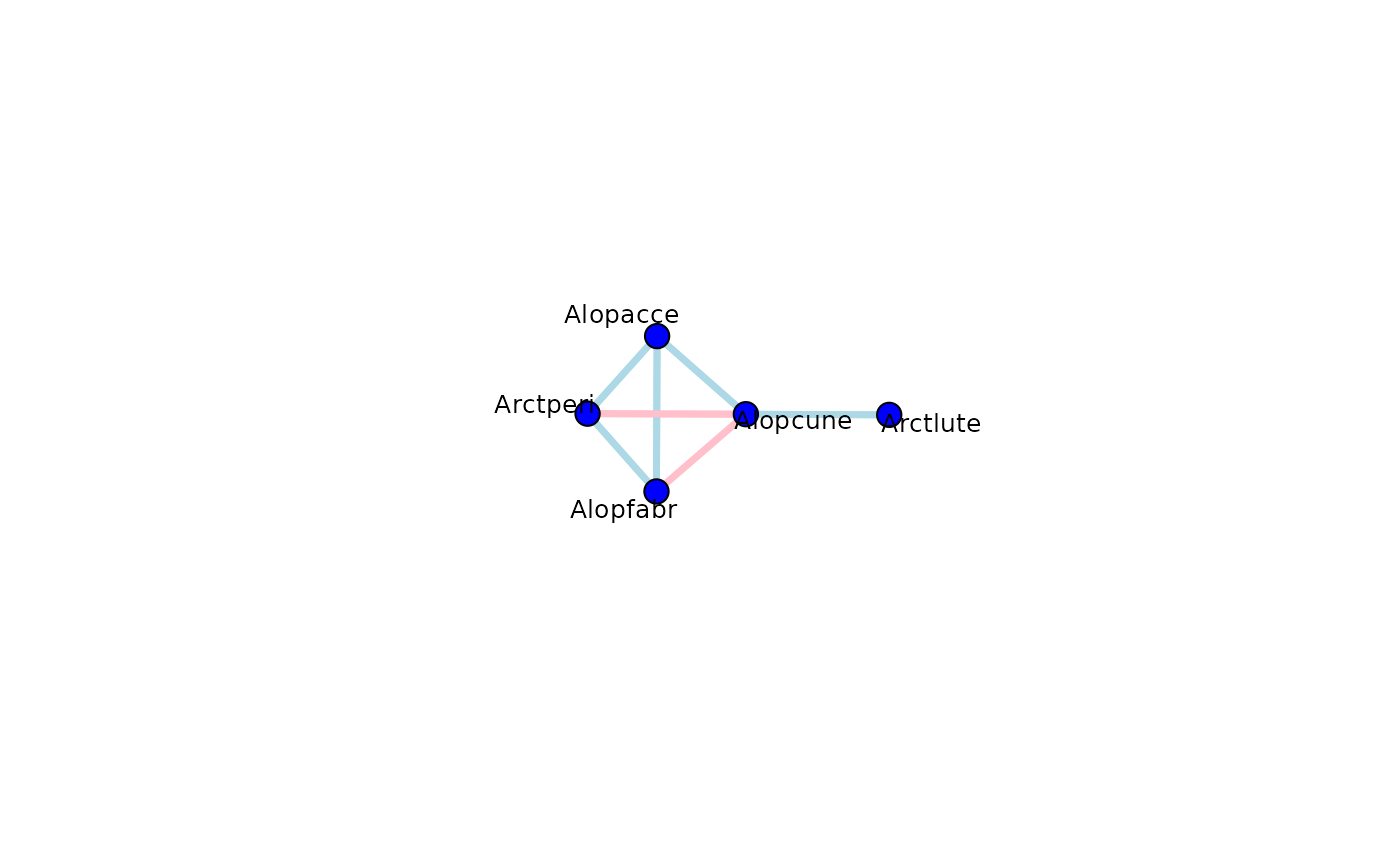
Examples

abund <- spider$abund[,1:5]
spider_mod <- stackedsdm(abund,~1, data = spider$x, ncores=2) 
spid_graph=cgr(spider_mod)
plot(spid_graph,pad=1)